@Johannes Kepler University (JKU), Linz: Motivated mainly by the apparent connection between AI technologies and approaches like modeling and NLP/LLM (Natural Language Processing/Large Language Models) and my discipline, ECM.
Part I Coming soon.
Coming soon.
Includes some WL (Wolfram Language). Let's always include some WL.
Seminar-presentation/Thesis I. Next up a practical component and the thesis itself.
Some housekeeping notes on my degree, and shorter tool-oriented posts about Wolfram Language, Prolog (!), and SMT2 for model checking and for planning are also here, whereas further Wolfram Language work is documented as part of my engagement at Wolfram Research.
rX Feed (really, notes on how to apply this stuff) and my formal thesis in its different parts, interlaced with these blog posts, become part of the same project, I find: I hope you have fun reading! All credit for the techniques presented goes to the authors. All errors in their presentation are mine. I am happy for you to get in touch for any comments, suggestions and any notes you have for me about the material.
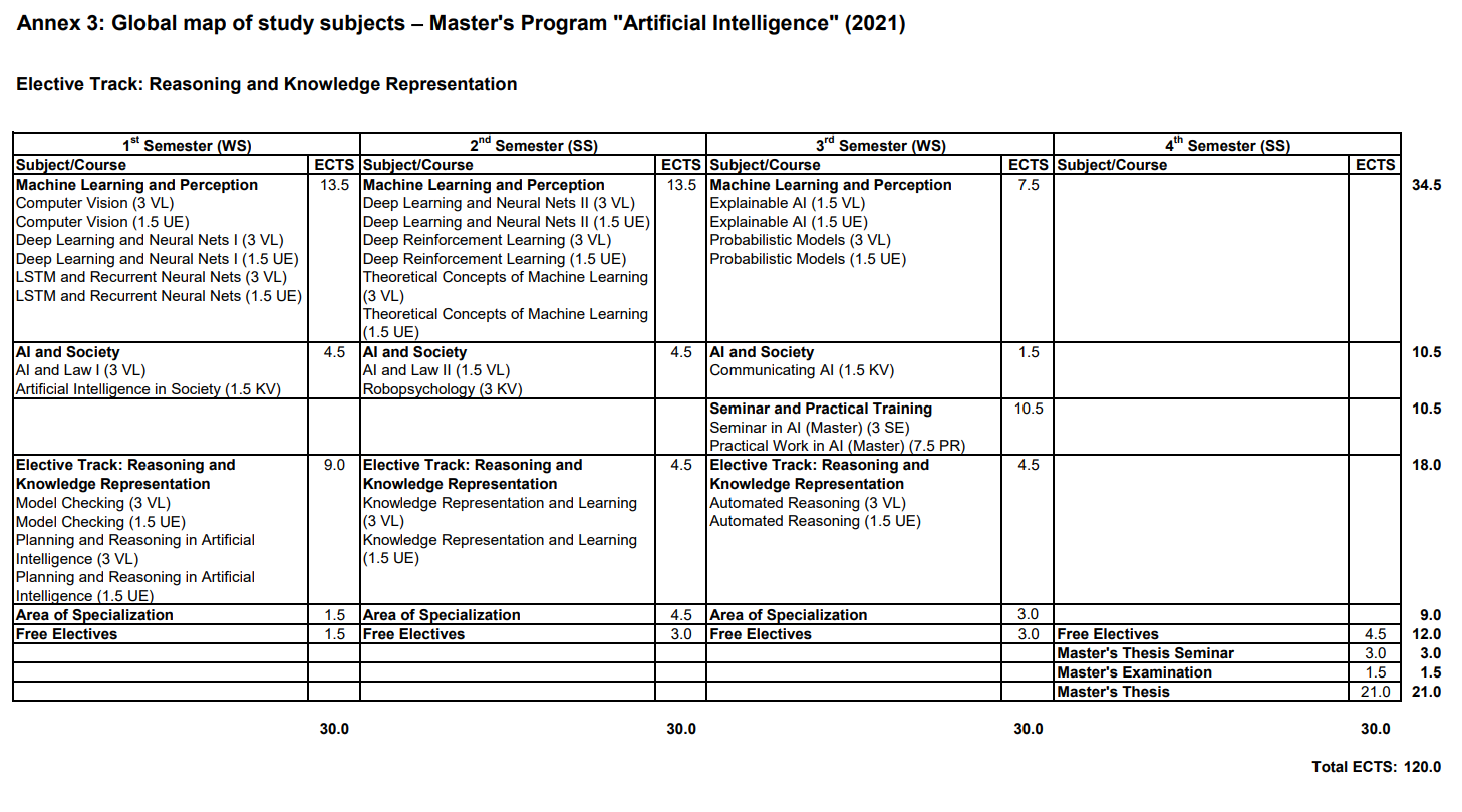
These Masters level studies are on-going (target December 2024), now full-time, and occurring in the context of the Symbolic/Mathematical Track @JKU's AI Masters in AI. The most up-to-date curriculum is listed in English and I also wrote a concept document for a potential Symbolic Computation direction of these studies post-Masters here in Linz, where however LLMs and are taking center-stage for now, as my Masters contribution to the Zeitgeist.
Repository on GitHub: for this Part I to a look at Deep Learning for Reinforcement Learning (RL), i.e. Deep Reinforcement Learning, I want to review some RL basics, largely following the well-tested Sutton and Barto text, ending on a note about planning vs learning and a focus on the foundational Bellman equation.
It's a core course for the Master's, treating a core AI datastructure so to speak, maybe as central as Convolutional Neural Networks, and at least framing the perspective on Transformers (where there is no separate course). After all, JKU's Sepp Hochreiter invented LSTM (Long-Short-Term Memory), but to go there, you need to start from RNNs (Recurrent Neural Networks) first.
This chain-like nature reveals that recurrent neural networks are intimately related to sequences and lists. They’re the natural architecture of neural network to use for such data.
RNN-Feats? Read The Unreasonable Effectiveness of Recurrent Neural Networks by Andrej Karpathy, maybe not so unreasonable in light of the quote from Chris Olah.
Let's try something to begin, though, before jumping into more background on RNNs generally, and LSTM specifically, right up to the 2024 xLSTM Story (DE-world currently).
I know Python is the default in many AI curricula nowadays, but tools like Wolfram Language (WL) can be more effective because they are more high level. It really depends on what you want to emphasize: are you interested in implementation details, or do you just want to work with the networks?
Let's try this Input:
(*recurrent layer acting on variable-length sequences of 2-vectors*)
lstm = NetInitialize@
  LongShortTermMemoryLayer[2, "Input" -> {"Varying", 2}]
(*Evaluate the layer on a batch of variable-length sequencesEvaluate the layer on a batch of variable-length sequences*)
seq1 = \{\{0.1, 0.4\}, \{-0.2, 0.7\}\};
seq2 = \{\{0.2, -0.3\}, \{0.1, 0.8\}, \{-1.3, -0.6\}\};
result = lstm[{seq1, seq2}]
Output:
\{\{\{-0.0620258, 0.0420743\}, \{-0.0738596,
   0.0826808\}\}, \{\{0.0240281, -0.00213933\}, \{-0.0691157,
   0.0852326\}, \{0.190297, -0.117645\}\}\}
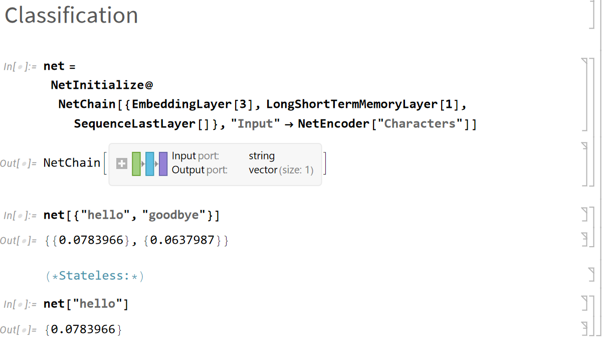
For something just a bit more complicated, let's produce a number for each sequence: this is what it would look like to chain up the layers in WL.
Input:
net = NetInitialize@
  NetChain[{EmbeddingLayer[3], LongShortTermMemoryLayer[1],
    SequenceLastLayer[]}, "Input" -> NetEncoder["Characters"]]
Output after the jump, in a repo I made for the demo notebook. If you don't want to download the notebook and boot up Mathematica, the output looks like this, however.
What follows is a small taxonomy of RNNs, centering on LSTM, with the formulas!
For the Jordan network, which is a type of recurrent neural network (RNN) that connects the output to the input of the network for the next time step, the equations are slightly different from those of LSTM-like networks we will look at in a moment.
$$ \begin{align} \boldsymbol{h}(t) &= \sigma\left(\boldsymbol{W}{h}^{\top} \boldsymbol{x}(t) + \boldsymbol{R}{h}^{\top} \boldsymbol{y}(t-1)\right) \ \boldsymbol{y}(t) &= \phi\left(\boldsymbol{W}_{y}^{\top} \boldsymbol{h}(t)\right) \end{align} $$
The point here is: weight sharing is emplyoed, that is, the same weights are used across time steps. R is the Recurrent Weight Matrix here.
The "simple recurrent neural network" as you sometimes see it called: Internal hidden activations are remembered, but hidden units loop only to themselves, not neighbors or any other units:
$$ \begin{align} \boldsymbol{h}(t) &= \sigma\left(\boldsymbol{W}_{h}^{\top} \boldsymbol{x}(t) + \boldsymbol{a}(t-1)\right) \ \boldsymbol{y}(t) &= \phi\left(\boldsymbol{V}^{\top} \boldsymbol{a}(t)\right) \end{align} $$
Do you spot what is moving in the formulas, as complexity and thereby expressivity is added?
$$ \begin{align} \boldsymbol{h}(t) &= \sigma\left(\boldsymbol{W}^{\top} \boldsymbol{x}(t) + \boldsymbol{R}^{\top} \boldsymbol{h}(t-1)\right) \ \boldsymbol{y}(t) &= \phi\left(\boldsymbol{V}^{\top} \boldsymbol{h}(t)\right) \end{align} $$
We arrive at the Fully RNN with recurrent hidden layers that are fully connected, so all the hidden units are able to store information, i.e. from previous inputs. There is a time lag to these connections, therefore.
Let's discuss the ideas on a high level.
The Autoregressive Moving Average (ARMA) model is a popular statistical model used for time series forecasting. It combines two components: Autoregressive (AR) and Moving Average (MA). The AR part involves using the dependency between an observation and a number of lagged observations. The MA part involves modeling the error term as a linear combination of error terms occurring contemporaneously and at various times in the past.
The ARMA model can be denoted as ARMA(p, q), where $$p$$ is the order of the autoregressive part, and $$q$$ is the order of the moving average part. The general form of the ARMA model is given by the following equation:
$$ X_t = \phi_1 X_{t-1} + \phi_2 X_{t-2} + \cdots + \phi_p X_{t-p} + \theta_1 \varepsilon_{t-1} + \theta_2 \varepsilon_{t-2} + \cdots + \theta_q \varepsilon_{t-q} + \varepsilon_t $$
Where:
The Nonlinear AutoRegressive with eXogenous inputs (NARX) model is a type of recurrent dynamic network that is particularly useful for modeling and predicting time series data influenced by past values of the target series and past values of external (exogenous) inputs. It is a powerful tool for capturing complex nonlinear relationships in time series data.
The Nonlinear AutoRegressive with eXogenous inputs (NARX) model can be represented as follows:
$$ y(t) = f\left(y(t-1), y(t-2), \ldots, y(t-d_y), u(t-1), u(t-2), \ldots, u(t-d_u)\right) + \varepsilon(t) $$
Where:
Finally, Time Delay Neural Networks (TDNNs) are a specialized form of neural networks designed to recognize patterns across sequential data, effectively capturing temporal relationships. TDNNs introduce a mechanism to handle time series or sequence data by incorporating time-delayed connections in their architecture. This allows the network to consider input not just from the current time step but also from several previous time steps, thus leveraging the temporal context of the data.
The operation of a neuron in a TDNN can be mathematically represented as follows:
$$ y(t) = f\left( \sum_{i=0}^{N} w_i x(t-i) + b \right) $$
where:
So much for further background on the architectural levels. Let's let the latter models especially serve as contextual notes, the goal always being to express connections across time steps. So far so good!
Unfolding the Network: The RNN is "unrolled" for each time step in the input sequence, transforming it into an equivalent feedforward network where each layer corresponds to a time step.
Forward Pass: Inputs are fed sequentially, and activations are computed across the unrolled network, moving forward through time.
Backward Pass: The loss is calculated at the final output, and gradients are backpropagated through the network, taking into account the impact of weights across all time steps.
Gradient Accumulation: Gradients for each time step are accumulated since the same weights are applied at every step.
Weight Update: The weights are updated using the accumulated gradients, employing optimization algorithms like SGD, Adam, or RMSprop.
- Vanishing and Exploding Gradients: These issues can significantly hinder learning, especially for long sequences. LSTM and GRU units are designed to mitigate these problems.
- Computational Intensity: Processing long sequences in their entirety for each update can be computationally demanding and memory-intensive.
- Truncated BPTT: This approach limits the unrolled network to a fixed number of steps to reduce computational requirements, though it may restrict the model's ability to learn from longer sequences.
BPTT enables RNNs to effectively leverage sequence data, making it crucial for applications in fields like natural language processing and time series analysis. We will pass by some important initialization, regularization, and other approaches and methods for the purposes of this summary post.
I'll refer to Dive Into Deep Learning's section on this topic.
Dive Into Deep Learning (ibid) has the idea:
... an approximation of the true gradient, simply by terminating the sum at $$\partial h_{t-\tau}/\partial w_\textrm{h}$$ . In practice this works quite well. It is what is commonly referred to as truncated backpropgation through time (Jaeger, 2002).
Here is a reference tutorial paper I really like by Herbert Jaeger, covering the method in some more detail and also presenting the material covered in this post from different angles.
RTRL is an online learning algorithm, which means it updates the weights of the neural network in real-time as each input is processed, rather than waiting for a full pass through the dataset (as in batch learning). This characteristic makes RTRL suitable for applications where the model needs to adapt continuously to incoming data, such as in control systems, real-time prediction tasks, or any scenario where the data is streaming or too large to process in batches.
The key feature of RTRL is its ability to compute the gradient of the loss function with respect to the weights of the network at each time step, using the information available up to that point. This is achieved by maintaining a full Jacobian matrix that tracks how the output of each unit in the network affects each other unit. However, this comes with a significant computational cost because the size of the Jacobian matrix grows quadratically with the number of units in the network, making RTRL computationally expensive for large networks.
Despite its computational demands, RTRL has been foundational in the development of algorithms for training RNNs, and it has inspired the creation of more efficient algorithms that approximate its computations in a more computationally feasible manner, such as Backpropagation Through Time (BPTT) and its various optimized forms.
RTRL is particularly valued in scenarios where it's crucial to update the model weights as new data arrives, without the luxury of processing the data in large batches. However, due to its computational cost, practical applications often use alternative methods that strike a balance between real-time updating and computational feasibility.
- BPTT (Backpropagation Through Time)
- Asymptotic Complexity: O(T * C) where T is the length of the input sequence and C represents the complexity of computing the gradients at a single timestep (including both forward and backward passes). The complexity scales linearly with the length of the input sequence but requires significant memory for long sequences.
- RTRL (Real-Time Recurrent Learning)
- Asymptotic Complexity: O(n^4) for a network with n units. This high computational complexity arises from the need to update a full Jacobian matrix tracking the dependencies of all units on each other at every timestep. It makes RTRL impractical for large networks despite its real-time learning capability.
- TBPTT (Truncated Backpropagation Through Time)
- Asymptotic Complexity: O(k * C) where k is the truncation length (the number of timesteps for which the network is unfolded) and C is similar to that in BPTT. TBPTT provides a more manageable and predictable computational cost, especially for long sequences, offering a practical compromise between computational efficiency and the benefits of temporal learning.
Let's dive into the formulas following the architectures approach from before.
$$ \begin{align} \boldsymbol{i}(t) &= \sigma\left(\boldsymbol{W}{i}^{\top} \boldsymbol{x}(t)+\boldsymbol{R}{i}^{\top} \boldsymbol{y}(t-1)\right) \ \boldsymbol{o}(t) &= \sigma\left(\boldsymbol{W}{o}^{\top} \boldsymbol{x}(t)+\boldsymbol{R}{o}^{\top} \boldsymbol{y}(t-1)\right) \ \boldsymbol{f}(t) &= \sigma\left(\boldsymbol{W}{f}^{\top} \boldsymbol{x}(t)+\boldsymbol{R}{f}^{\top} \boldsymbol{y}(t-1)\right) \ \boldsymbol{z}(t) &= g\left(\boldsymbol{W}{z}^{\top} \boldsymbol{x}(t)+\boldsymbol{R}{z}^{\top} \boldsymbol{y}(t-1)\right) \ \boldsymbol{c}(t) &= \boldsymbol{f}(t) \odot \boldsymbol{c}(t-1)+\boldsymbol{i}(t) \odot \boldsymbol{z}(t) \ \boldsymbol{y}(t) &= \boldsymbol{o}(t) \odot h(\boldsymbol{c}(t)) \end{align} $$
The Vanilla LSTM, distinguished by its three gates and a memory state, is a staple variant in the realm of Long Short-Term Memory networks. It stands out for its ability to selectively preserve or ignore information, making it adept at managing memory cells amid potential distractions and noise. This selective filtering results in a highly non-linear dynamic that equips the LSTM to execute complex functions effectively.
Here's an overview of the Vanilla LSTM's operation, highlighting its components and their respective functions:
x(t)): Incoming data at each time step, transformed into cell input activations (z(t)) through a non-linear function (g(·)), typically the hyperbolic tangent (tanh).i(t)): Utilizes a sigmoid function to filter (z(t)), allowing only relevant information to pass through based on the current context.f(t)): Also employing a sigmoid function, it determines the proportion of the previous cell state (c(t−1)) to retain or discard, enabling the cell to forget irrelevant past information.c(t)) is formed by an element-wise addition of the product of the input gate and cell input activations (i(t)⊙z(t)) with the product of the forget gate and the previous cell state (f(t)⊙c(t−1)), effectively updating the memory with relevant new information while discarding the old.o(t)): The final step involves squashing the memory cell's contents into a numerical range via a cell activation function (h(·)) and then filtering this through an output gate. This process yields the final memory cell state activation (y(t)), ready for the next computational step or to serve as the output.This structured approach allows the Vanilla LSTM to adeptly navigate through time series data, learning from long-term dependencies and making it a powerful tool for a wide range of sequential data processing tasks.

Figure from K. Greff, R.K. Srivastava, J. Koutnik, B.R. Steunebrink, J. Schmidhuber. IEEE Transactions on Neural Networks and Learning Systems, Vol 28(10), pp. 2222–2232. Institute of Electrical and Electronics Engineers (IEEE). 2017.
Focused LSTM: No forget gate and fewer parameters than Vanilla LSTM.
Lightweight LSTM: The Focused LSTM without output gates. (Has Markov properties*.)
(*The Markov property is a fundamental concept in the theory of stochastic processes. It refers to the memoryless property of a process, where the future state depends only on the current state and not on the sequence of events that preceded it. There are several types.)
Gated Recurrent Unit (GRU)
A slightly more dramatic variation on the LSTM is the Gated Recurrent Unit, or GRU, introduced by Cho, et al. (2014). It combines the forget and input gates into a single “update gate.” It also merges the cell state and hidden state, and makes some other changes. The resulting model is simpler than standard LSTM models, and has been growing increasingly popular.
From Chris Olah’s Understanding LSTM Networks: great diagrams there.
Regardless of architecture, and since a lot has been written to explain LSTMs from the ground up, I would like to clear up the blocks you might face if you are similar to me, as you try and understand the approach.
I can really recommend StatQuest if you want a video, but you have to like the StatQuest presentation style ("Bam").
See Ticker Steps, Negative Gate Biases, Scaled Activation Functions, etc. in The Sorcerer’s Apprentice Guide to Training LSTMs by Niklas Schmidinger.
For another day: JKU in the headlines, precisely on topic, but what's the idea? I think this is not yet out of the bag but will be soon, providing an opportunity for another post here. At the core, this is about LSTM vs Transfomers however and sounds like something hybrid.
The transformer computations increase quadratically according to the text length. By contrast, xLSTM calculations increase in a linear manner only, along with the text length, thereby using less processing power during operation. As complex tasks require more text for both the task description and the solution, this is a great advantage. Fortunately, xLSTM can, for example, facilitate industrial applications, especially if transformer models are too slow. Similar to transformer models, xLSTM has a phonetic memory. The algorithm is, however, equipped with an additional component that results in a closer resemblance to human verbal working memory, making the xLSTM algorithm much more powerful.
I am excited to catch wind of the story directly as it unfolds at JKU.
The remaining sections in this page deal with all other areas of my degree including other parts of the Symbolic track in Linz, already completed and outlined towards the end of the page.
As my thesis approaches a writing-stage, I start to think about the tetris-like putting together of my thesis committee, following this guideline (online in full (EN)).
As part of the oral examination, the student will be asked to create a 3-member examination committee consisting of a committee head (member 1) and two additional members (members 2 and 3). This first committee member may not be a thesis supervisor and will preside over the oral defense. The second committee member will conduct an examination in the subject area of “Machine Learning and Perception”. The third committee member will conduct an examination in regard to the selected elective track. The thesis supervisor should also be a member of the committee. Whereas two committee members may be from the same institute, all of the committee members should not be from the same institute.
Is this task AI/Symbolically solvable? A neural network could do it, we can be sure of that.
The ca. one-hour long exam remains for me to do, not the AI, and is about my Master's thesis, with a grade provided by member 1 in the above. Members 2 and 3 cover the required and elective coursework (according to a track, Symbolic in my case). Because I have two supervisors and it seems at least one of them (conceivably both) need to be part of the examination, I see how these slots fill up and decide subject areas in terms of the examiner for me: my supervisors come from the machine learning and the knowledge processing institutes respectively, where machine learning constitutes the core, required coursework and knowledge processing is taken to be part of the symbolic track (where I actually would have liked a cross-over to Wolfram Language and RISC topics, but cannot cover these in this view - except maybe if there is no need to task all supervisors to the examination table!) so it looks like this is where I am headed, to exit my degree (in style) eventually.
Mysterious member No 1 remains to be chosen! I wonder if this one might be offered by the Insitute of Integrated Study, see below details on the thesis' genesis.
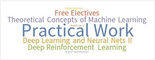
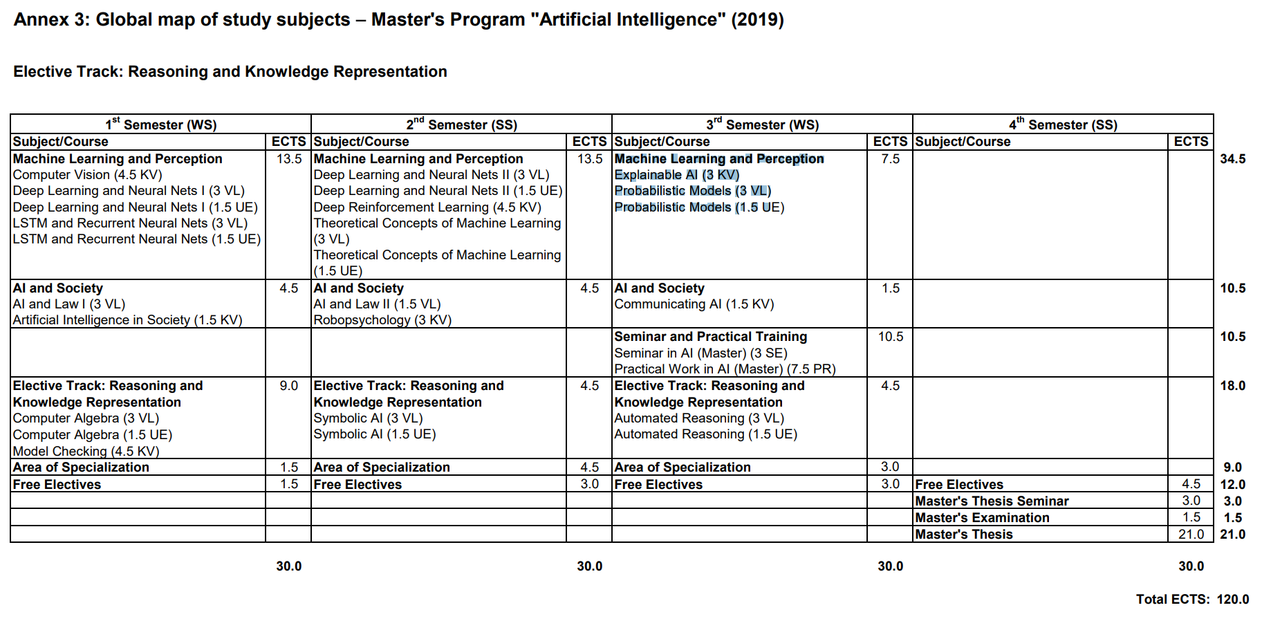
So the matter is complicated by a slight difference between the 2019 and the current 2021 curriculum (it is 2024 now and there is a delay between the given years and the years studied by: I am studying by the 2021 curriculum, I believe (!), but started by the 2019 curriculum - will need to check the details with the studies admin) but ok, let's not get weighed down here: by the 2019 curriculum and according to my original idea for this studies, subject to some slight shifting of coursework according to interest or lack thereof (sorry, looking at you, Computer vision), here are some nice Wolfram Language word clouds with the credit-weighted course titles, listed by semester.
Please don't ask why I do things in complicated ways! During my SE Bachelor's I enrolled in university coursework from the AI curriculum, both Bachelor's and Master's level, and then formally entered into the Master's on the basis of my college Bachelor's - requiring some preliminary coursework from the AI Bachelor's. All while already working after college, which yes, did add a stress factor, so if you are planning a similar route, probably best to go it more linearly. But sometimes these things just come a certain way: in addition to the following timeline and work officially credited to the Master's I actually did a lot of Bachelor's level courses from both the JKU AI and CS (or Informatics, as Austrians like to say) Bachelor's, before at arriving at my model of combining skills-based learning at Hagenberg with semi-direct entry to a science-oriented Master's.
So yes, please don't ask why I do things in complicated ways!
I already started on some Master's level coursework too here, Model Checking, some Computer Vision (lecture requirement), Basic Methods of Data Analysis (from the Bachelor's actually), AI in Medicine (short course at the Medical Faculty in Linz).
Also did Knowledge Representation and Reasoning (formerly Symbolic AI) at the Master's level here.
Curricular ideal (here's a magical German term for you: "Idealtypischer Studienverlauf" ... ideal-typical (?) course (trajectory) of studies):
Model Checking was already done in Pre I, note on Computer Algebra: replaced by Planning and Reasoning in AI in the 2021 curriculum. I took the Planning course, see the following word cloud, but still want to try and integrate Computer Algebra with my Master's as well, if possible: I am already in touch with the studies admin about this now.
So, the Jack-actual (Computer Vision will be done in Semester III, which I am ok with, so I consider my target reached):
The upcoming semester, let's see if I can follow the ideal.
Actually, I already know I am doing my Practical Work Component this semester, so that already breaks with the ideal ...
Also Symbolic AI (now called Knowledge Representation and Reasoning) was already completed in Pre II: so, in other words, shooting beyond ideal here, for my target.
Once again an ideal:
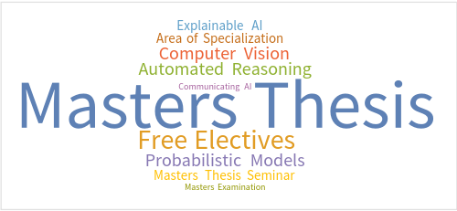
This might be a lofty goal ... I already completed Practical Work and Seminar at this point, and need to wrap my Master's thesis (pulling from the intended Semester IV), but still need to do the Computer Vision component (technically only the exercise, the lecture was done in Pre I actually) on the other hand, so:
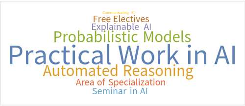
Automated Reasoning is listed for this semster (2019 version), and is only offered this semester currently, along with Computer Algebra (but this one is not required in the 2021 curriculum anymore, just a nice course).
Basically only if needed for anything else than the following curricular ideal, where I already completed everything if I stay on target (then I would be doing my exam, see above, in the spring, which could be a nice timeline too): this would be a whole semester reserved for Masters Thesis (writing), Seminar and Exam. We'll see.

12 credits to fill according to both curriculum versions below, CAN be taken from the AI Masters prerequisite Bachelor's level coursework too. (See Pre I and II above.)
9 credits to fill:
(Looks like cannot be granted because AI Masters prerequisite Bachelor's level coursework is not elgible in this category: tough bureaucracy!)
So then, I can offer:
Oh, that's already 9! There are some other courses of interest available actually (looking at you, Semester III and Shadow Semester IV), see the JKU AI Master's handbook for a current list.
Just kind of happened:
Also
probably not needed, along with a couple more exercises and lectures from the AI Bachelor's which will probably not be credited towards my Master's, which is only okay in a county where the higher ed price tag goes to zero/see above.
For a rounded Masters Thesis, on an ECM-AI topic naturally, a comparative exploration of Finetuning especially opposite In-Context Learning approaches is the goal, starting with a seminar on a current paper and a company-affiliated (some more news to follow) practical work, all on the topic of making PDF-documents accessible.
Very related to the EU Context: The European Accessibility Act (EAA) is an EU Directive that sets binding accessibility goals to be achieved by all the member states, to be implemented by 2025.
(Masters-)Project is a Go! I even managed to get some Borges in, see slides three and four in the presentation.
Delivered on December 11th, 2023, to IML (Machine Learning Insitute) at Johannes Kepler University.
TBD, e.g. a standard software component to check and transform PDFs to accessible formats in a fully automated fashion.
TBD fully, most likely a comparison with Finetuning appraches incl. use of open models like Llama.
This could be a real world application too, clearly, since the basic functionality can be distributed by API with customization and standard software modules, as might be done for practical thesis work, on top: This idea also provides a clear delineation between data-oriented service (transformation to barrier free documents) and a module that would be implemented for a company in practical work, with loss of rights to such a module.
For this project, full repo available, I was more involved in the SMT2 (Satisfiability Modulo Theories Version 2) side, something I could imagine tying into (Python) projects in the future, for validation and checking (and here planning) purposes - so I ended up exploring interfacing modalities, here the digram overview for Part 2 of the project, the SMT-part.
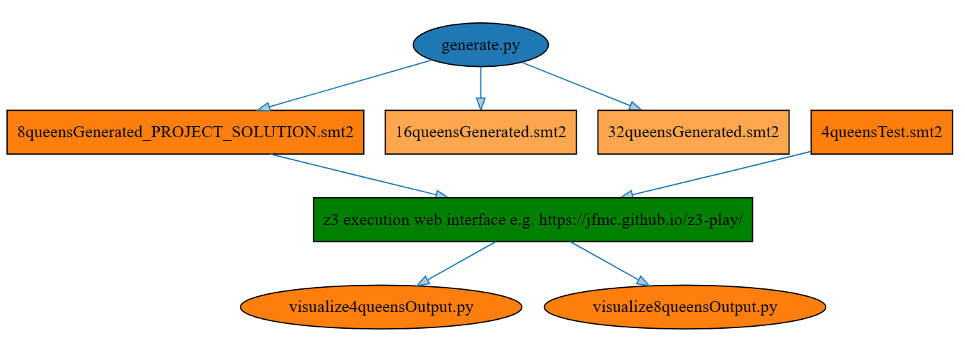
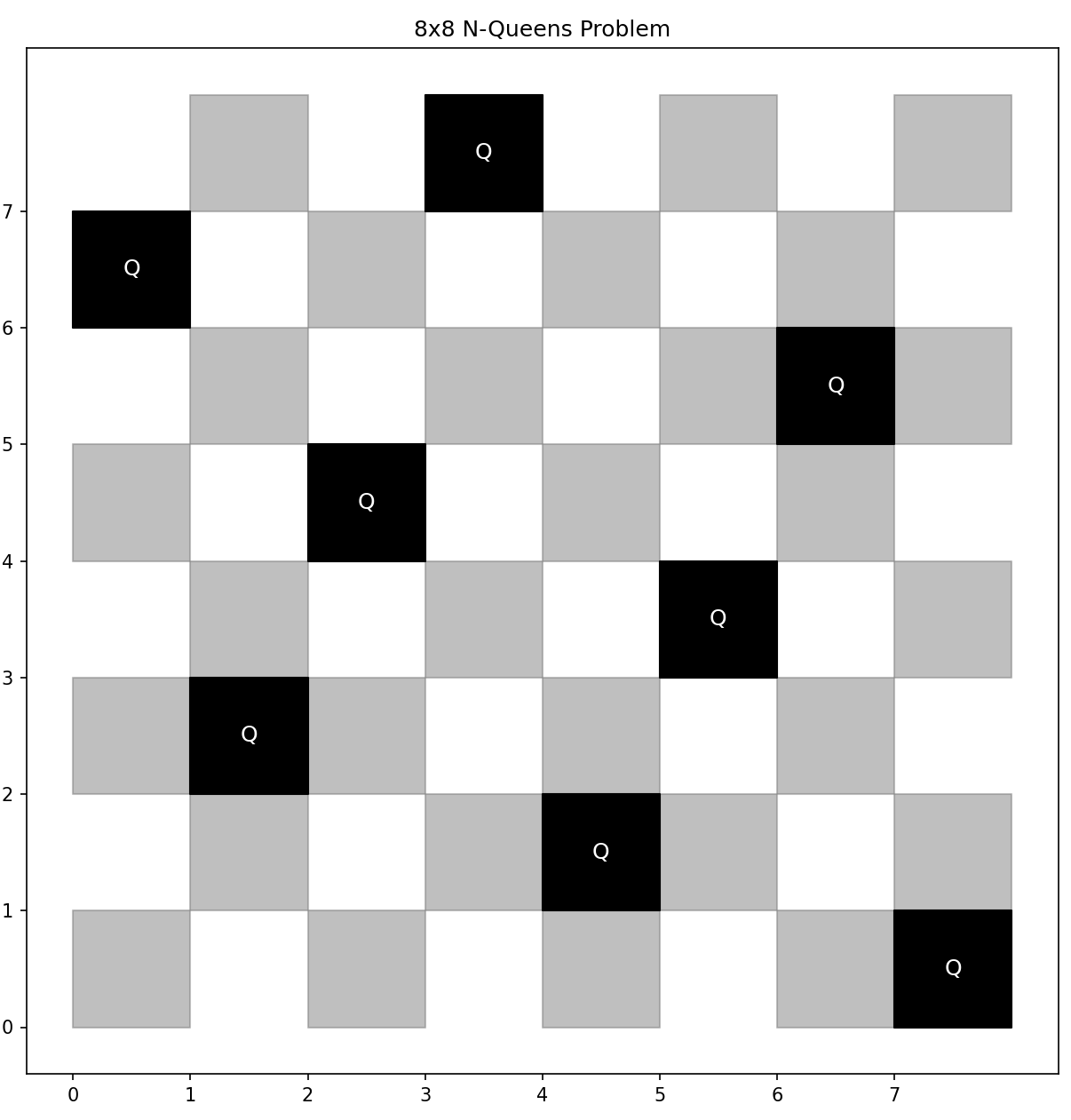
The actual application is the N-Queens Problem, specifically the 8x8 version, where my solution actually implements a generator code file for generic problem sizes, together with MatPlotLib visualization actually:
Part 1 is a Limboole implementation, see the repo: I like Limboole because it is a JKU project, as "a simple tool for checking satisfiability respectively tautology on arbitrary structural formulas, and not just satisfiability for formulas in conjunctive normal form (CNF), like the DIMACS format, which the standard input format of SAT solvers. The tool can also be used as a translator of such structural problems into CNF." Quoted from the JKU Insitute for Formal Models and Verification
A little more on JKU institutes actually: This concludes my Masters work in the JKU Symbolic AI Institute, where the other course was Model Checking. Work with FAW, the institute, (Knowledge Representation and Reasoning) is also already completed, apart from the Masters Thesis which will be co-supervised by FAW (together with the Machine Learning Institute): leaving Automated Reasoning and Computer Algebra for 2024, both located at RISC, which I hope to connect to from my work with Wolfram Language.
Taken together, this is a symbolic counterpoint to my thesis direction working in language models and applications, reflected in my resarch (rX) feed going forward.
More details on my work in symbolic computation and Wolfram Language on my Wolfram page, touching on my consulting work for the company as well.
I was a grad student participant in the 2023 Wolfram Summer School (WSS) three weeks in June and July 2023.
Somehow intertwined with this, for me subjectively: the Nativist/Symbolic vs. Empiricist/Neural Networks debate, see Does AI need more innate machinery? (Mathematica is a symbolic computation tool.)
My main reason for WSS was a turn to further university level math and the realization that I want a standard tool to do some of the work. More on a concept for these potential studies in Linz/Hagenberg (Austria, Software Engineering and AI studies) incl. a view towards a Symbolic Computation PhD (again, writing it out as a potential long-term view).
To connect Wolfram/Mathematica with my Masters-level courses: Computer Algebra and Automated Reasoning (see concept document, these are the core RISC courses in my study track) require/substantially benefit from Mathematica. Here, for now, is the poster output of the summer school.
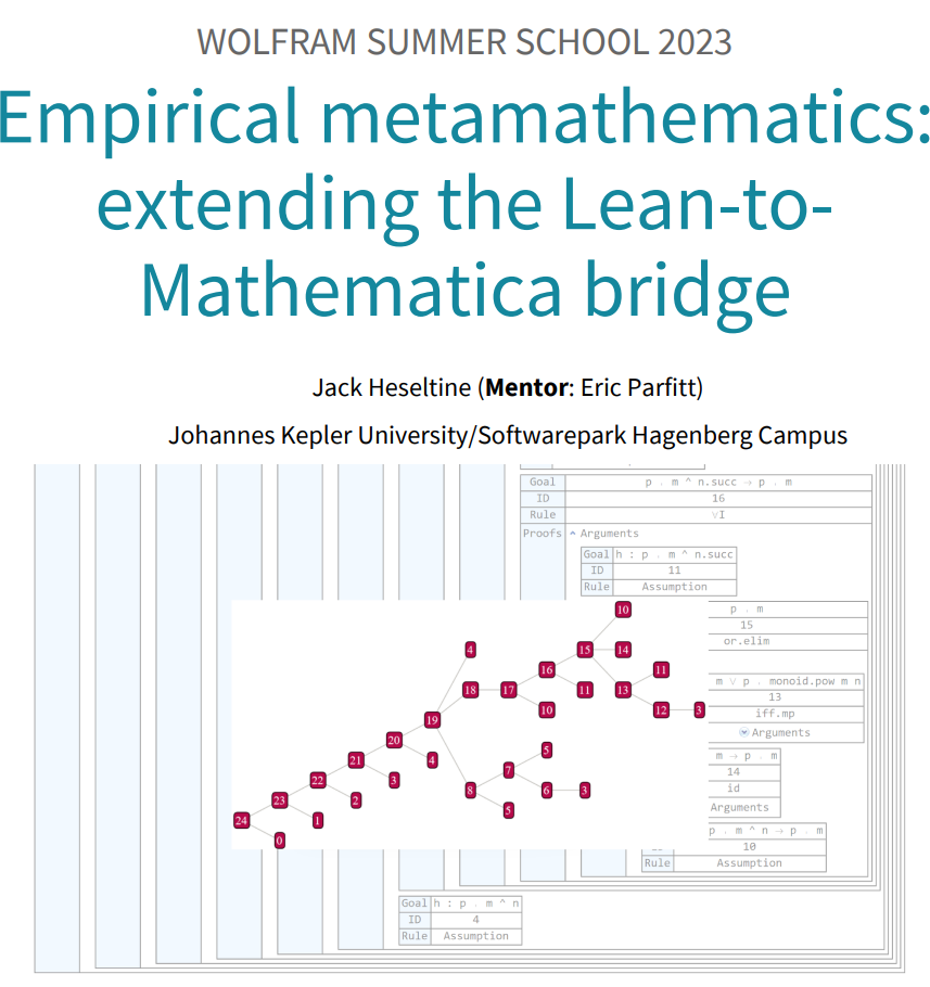
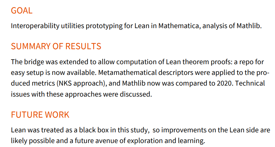
The final output of the school was a community post and presentation, forthcoming as a publication in the 2023 Wolfram Summer School Proceedings: I also handed in results and further study for my studies in Software Engineering at Hagenberg, see the Software Engineering page about the thesis this became.
This is an example where the stopping criterion is needed for a recursive call, for instance:
lastElement([E],E). % (1)
lastElement([K|R],E) :- lastElement(R,E). % (2)
In any case a program like the above is built up, involving facts (1, the %-sign makes a line comment) and rules (2), making for a knowledge base that can the be queried or used to proove certain statements, also encoded in prolog. The tool used was SWI Prolog. The above code snippet also shows the typical use of recursion to encode iteration.
In a project team of three, I tackled a solver for the game Ruzzle (a bit like scrabble) with possible uses as a challenger AI or general solving tool. (Github has the code, and there's slides to get an overview over the project too, presented at Johannes Kepler University on April 25th, 2023.)
The full project is on GitHub, but the principles can be summed up in a paragraph: Satisfiability Modulo Theories (SMT) is a growing area of automated deduction with many important applications, especially system verification. The idea is to test satisfiability of a problem formula against a model. Here's an example: a C-program is the model, some bug encoded into an formula is to be checked. If we get a satisfiable result, that is bad, because that means the bug is possible against this particular C-program. So what you are usually after in a verification task is actually an unsat(isfiable) result.
$$ {\displaystyle {\overline {a\land b}}\equiv {\overline {a}}\lor {\overline {b}}} $$
(declare-fun a () Bool)
(declare-fun b () Bool)
(assert (not (= (not (and a b)) (or (not a)(not b)))))
(check-sat)
Result:
unsat
The unsat result means that the negated (!) proposition (De Morgan's law) is not satisfiable: it is true.
The concrete application was a numerical pad implementing a locking system (think something like a safe), coded up with C, and the task was to check for bugs. The final approach chosen by me and a project team of another person was to encode eight separate SMT LIB (SMT-standard language) files to run with Z3, Microsoft's SMT solver. This allowed us to rule out certain buggy behaviors to help locate the actual possible bug in the C program.